Real-time chunking: the parts that trip you up

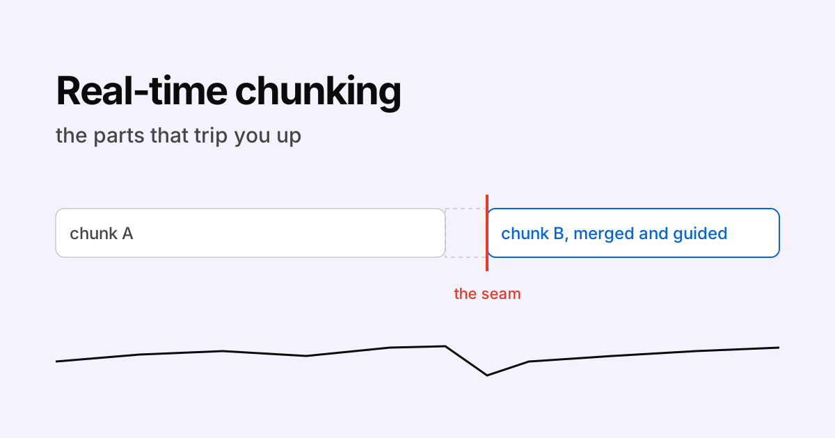
Real-time chunking, RTC, is the trick that lets an action-chunk policy such as pi0.5 keep the robot moving while the next chunk is still being computed. I spent a week with it: reading the paper, reading LeRobot’s open-source implementation line by line, and working out why an inference engine built from an ONNX export can carry one version of the guidance step but not the other.

I got the picture wrong several times, and every wrong picture was a natural one to hold. This post walks through the six places where it happened, with figures you can push around, so you meet the pitfalls here rather than on a robot.

The paper is Black et al., Real-Time Execution of Action Chunking Flow Policies (2025). LeRobot’s implementation is src/lerobot/policies/rtc/modeling_rtc.py in the lerobot repository. I assume you know what a VLA is and that pi0-style policies emit a chunk of future actions rather than one action at a time.

1. The ε in the loss is not an error

The action expert in pi0-style policies is a flow-matching model. Its training loss is one line:

x_t = t·ε + (1−t)·a        L = E ‖ v_θ(x_t, t, o) − (ε − a) ‖²

Every symbol in it has a name that collides with something from RTC, so here is what each one is. a is a real chunk from the dataset. ε is a block of Gaussian noise the same shape as a chunk, drawn fresh for each example. It is not an error term. t is a noise level between 0 and 1, drawn at random per example: at 0 the mix is the real chunk, at 1 it is pure noise. x_t is the mix, a point on the straight line from the chunk to the noise. o is the observation, images, state and prompt. v_θ is the network’s output, a block the same shape as the chunk.

The target the network must hit is ε − a, the direction from the chunk to the noise along that straight line. It is the same at every point of the line, so it does not depend on t. That is the whole reason one network can serve every denoising step later: whatever level of noise it is handed, the right answer is the same arrow.

Figure One training example, one noise level

x_t = 0.50 · eps + 0.50 · a  ·  target = eps − a (does not depend on t)

Eight rows of a single joint's real chunk drawn as a smooth line, eight noise values drawn as hollow circles, and the mixed point x_t sliding between them as t changes. Arrows from each real value to its noise value show the regression target eps minus a, which stays the same at every t.

The figure has one joint and eight rows to keep it readable. Slide t from 0 to 1 and watch the blue mix travel from the black chunk to the hollow noise points. The red arrows, the regression target, never move.

2. The field does not change. The point does.

At inference the loss is run backwards. Start from a block of pure noise, ask the network for the velocity, move a tenth of the way along it, ask again from the new position, ten times. The output of the network is best thought of as a vector field: for any block at any noise level, it says which way and how fast to move.

The pitfall is to hear “the velocity is recomputed at every step” and picture the field itself changing, or worse, the weights adapting. Neither happens. The weights are frozen. The field is whatever the trained network says, everywhere, forever. What changes is where you read it, because the block moved and the level dropped.

Figure The field does not change. The point moves.

At t = 1 the field points toward the average plan. Press Step to take one Euler move x ← x − 0.1·v.

A grid of small arrows over a plane, two target points marked as the data modes, and a moving point that starts at a noise sample and takes ten Euler steps along the arrows toward one of the modes. At each step a red arrow shows the velocity at the point and a hollow marker shows the clean estimate.

This toy has a two-number chunk and two possible plans, so the field can be drawn exactly: it is what a perfectly trained expert would output for that dataset, no network needed. Press Step and watch the red arrow at the point change from one step to the next. The grid around it is the same field, read at a lower t. The hollow marker is the clean estimate, x − t·v, the network’s running guess of where the block will land. Keep that marker in mind: guidance is built on it.

3. Merging without guidance is not real-time chunking

A chunk of a few dozen rows at 30 Hz lasts about a second. An inference takes a few rows’ worth of time. If the next request only goes out when the chunk runs dry, the arm holds for those rows at every boundary. That is the hard switch, and its cost is a stall, not a kink: the new chunk was inferred from the state the arm is actually in, so its first row starts near where the old one stopped.

Real-time chunking launches early, while some rows are still unplayed, and when the reply lands it drops the rows that were played in flight so the new chunk continues from the row that is due now. That is the merge. The pitfall is to call the merge “RTC” and expect smoother seams from it. It removes the stall and nothing else. The two rows that now meet at the seam were computed from observations a few rows apart by two independent samples of the model, and nothing ties them together. Expect that seam to be rougher than a hard switch, not smoother: at a hard switch the new row 0 is at least anchored to the current state.

Figure What actually meets at the seam

Launch with 8 rows left, reply after 3: A rows 30–34 never play, B rows 0–2 dropped, seam joins A29 → B3. Seam step shown: 5.0× the interior step (illustrative).

Two rows of cells for chunk A and chunk B on a shared time axis, showing which rows play, which are in flight during inference, which are never played, which are dropped by the merge, and where the executor holds. Below, a single joint's commanded position with the step at the seam drawn as a multiple of the ordinary step. Controls set the prefetch lead, the inference delay in rows, and whether the merge runs without guidance or with it. Seam step sizes are illustrative.

What ties the two plans together is guidance, the second half of the paper, and the rest of this post is about how it works and where it can run.

4. Guidance does not paste rows. It steers every step.

Here is the idea from the paper in one sentence. Some rows of the new chunk are already decided: the ones the executor will play before the new chunk can take over, plus a few more we would like to keep consistent. Treat them like the known pixels in image inpainting, and let the model fill in the rest so it blends.

The pitfall is the word “inpainting”. It suggests that the old rows are copied into the new chunk. Nothing is copied. Guidance is a nudge applied inside the sampler, at every one of the ten denoising steps, to the velocity. The block is compared to the old tail through the clean guess from section 2, the gap on the held rows is measured, and the velocity is edited so the next Euler move shrinks that gap. Then the network is called again, from the corrected block.

The paper and LeRobot share every part of that step except one. The paper computes the push by carrying the gap back through the action expert: how would the clean guess change if the noisy block changed, through the network. LeRobot’s processor calls the same autograd function, but read the code carefully. The velocity is computed before the input is marked differentiable:

with torch.enable_grad():
    v_t = original_denoise_step_partial(x_t)
    x_t.requires_grad_(True)
    x1_t = x_t - time * v_t
    err = (prev_chunk_left_over - x1_t) * weights
    correction = torch.autograd.grad(x1_t, x_t, err.clone().detach())[0]

Because v_t carries no dependence on x_t at the moment the gradient is taken, the only path from x1_t back to x_t is the direct term, and the gradient call returns err unchanged. The Jacobian is, in effect, the identity. Whether that was the intent is not something the code can tell you. What it does is clear.

Figure One guided denoising step, layer by layer

Scroll or press Next to walk one denoising step.

1. 1. Start of step k

   The block x_t, mostly noise at k = 0. Rows 0 to 2 are the held rows: they will be executed before the new chunk can take over, so the new plan must agree with the old tail Y there. Y is the black tick on each held row, already shifted into the new inference’s frame.

2. 2. Forward pass

   The expert reads the block, the observation and t, and returns a velocity for every row, the grey arrows. This is the only network call in the step. Nothing about guidance has happened yet.

3. 3. Clean guess

   x̂₁ = x_t − t·v: where the block would land if the current velocity were followed to the end. The hollow markers. No extra call, it is arithmetic on what the forward pass already returned.

4. 4. Gap on the held rows

   e = W ⊙ (Y − x̂₁), the red segments. Zero on the free rows by construction, because W is zero there.

5. 5. Push

   LeRobot: c = e, the gap itself, on the held rows only. The free rows get nothing. The paper: c = Jᵀe, the gap carried back through the expert, so every row gets a share sized by how much it influences the held rows. Use the toggle above the figure to compare.

6. 6. Velocity edit and Euler move

   v′ = v − g·c, then x ← x − 0.1·v′. The held rows slide toward Y by a tenth of the gain times the gap; with the cap at 10 and k = 0 that is the whole gap. The weights never changed. Only the block did.

7. 7. Next step, ten times

   The next forward pass sees the corrected held rows and, through attention across the chunk, predicts free rows that fit them. That is how LeRobot’s version gets its consistency, one step late; the paper’s push had already moved the free rows. When the tenth step ends, the merge drops the rows that were played in flight and the rest is published.

A block of eight rows of one joint drawn as horizontal bars. The first three rows are marked as held, with a tick for the old tail's value on each. As the steps advance, grey velocity arrows appear on every bar, hollow markers show the clean guess, red segments show the gap between the guess and the tick on the held rows, blue arrows show the push, and finally the bars move. With the LeRobot toggle the blue arrows appear only on the held rows; with the paper toggle they appear on every row, largest on the held ones.

Two things I had wrong. First, I assumed the paper changes the weights at inference. It does not; it differentiates with respect to the block, the same way you backpropagate to an image to see what a classifier responds to, and the weights are untouched. Second, I thought the paper “solves for the input that would have produced the corrected guess”. It takes one step of steepest descent on the held-row gap, in block space; nothing is inverted. LeRobot’s version is the same step with the network’s part of the sensitivity dropped, which is why its push lands only on the held rows.

5. The weight is not the timestep, and it is not a ramp

LeRobot exposes one number for the strength of guidance, max_guidance_weight, and it is tempting to read it as the strength of the pull, or to assume the pull grows step by step until the held rows match exactly at the end. I held both of those pictures. Both are wrong, and the formula settles it faster than any summary of it.

The pull at step k is a gain that follows a closed form in the step fraction τ = k/10, clipped at the cap. Read the formula: it is symmetric in τ and 1 − τ, so it is large at the first steps, smallest in the middle, and large again at the last. The cap is the only place where two settings of max_guidance_weight differ.

Figure The gain per denoising step

cap 10 limits steps 0, 1, 9 · fraction of the gap closed per step: 1.00 0.91 0.43 0.28 0.22 0.20 0.22 0.28 0.43 0.91

Ten bars, one per denoising step, showing the guidance gain. The bars are tall at steps 0 and 1, fall to a minimum of 2 at step 5, and rise again to the cap at step 9. A dashed line shows the same schedule with a cap of 5 for comparison. A slider changes the cap; the readout lists which steps the cap limits and the fraction of the gap closed at each step.

Because the block moves a tenth of the edited velocity per step, the fraction of the held-row gap closed at a step is a tenth of the gain. With the cap at 10 that is the whole gap at step 0, a fifth at step 5, and nine tenths at step 9. With the cap at 5 the first two steps and the last close half instead. Every other step is identical. If you ever compare cap 5 to cap 10, remember you are comparing three steps out of ten.

The second knob is which rows are held, and LeRobot builds it fresh before every inference in get_prefix_weights.

Figure Which rows are held, and how hard

exp: 1.00 1.00 1.00 0.63 0.37 0.19 0.08 0.02 0.00 0.00 0.00 0.00

A line chart of the guidance weight per row for the first twelve rows of a chunk. Rows before the inference delay have weight 1; from there the weight falls to zero at the execution horizon. Radio buttons switch between the zeros, linear, exp and ones schedules; sliders set the delay and the execution horizon.

Three knobs, then: the per-row weights say which rows are tied to the old tail and how tightly, the gain says how hard the tie is pulled at each denoising step, and the cap clips the gain. “Guidance off” is just the zeros schedule, which holds only the rows the merge is going to drop anyway.

6. The paper’s version cannot ride in an exported engine

Suppose you want to deploy the policy through TensorRT or a similar runtime. You export the sampler to ONNX by tracing it: run it once, write down every tensor operation that executed. Matmuls, attention, the subtraction that makes the clean guess, the multiply that makes the gap. The ten denoising steps are unrolled, so the file holds ten copies of the action expert. Then the runtime compiles that record into kernels.

The pitfall is to blame quantization. FP8 and BF16 have nothing to do with it. A gradient call is simply not a tensor operation. When PyTorch computes a gradient it does not read a list; it walks, backwards, the derivative records it kept while the forward pass ran, and that recorder and that walker live inside PyTorch. ONNX has no node that says “differentiate this”, so the tracer writes nothing down at that point, and the runtime compiles only what was written down. The hole is exactly where the paper’s push would be.

Figure What the exporter records

Press Trace to walk the operations in the order the exporter meets them.

Two columns listing the operations of one guided denoising step, one for the paper's implementation and one for LeRobot's. Every operation is marked as recorded by the ONNX exporter except the paper's push, an autograd call, which is marked as having no operator. A button walks the list the way the tracer does.

LeRobot’s push is a subtraction and a multiply, forward operations both, so it survives the export unchanged. That is the thing I understood last: the identity version is not a choice you would make on a whiteboard, but it is the one that can be traced into a graph. Quantization is a second wall behind the first: even if you hand-built the backward pass of the expert out of forward operations, doubling the graph ten times over, there is no low-precision recipe for a backward pass through attention, and you would have to re-verify the engine against eager PyTorch from scratch.

What I would tell myself a week ago

• ε is noise. The regression target is ε − a, the same at every noise level.
• The field is the frozen network. The velocity changes step to step because the block moved and t dropped.
• Prefetch and merge buy cadence and nothing else. Without guidance, expect the seam to be worse than a hard switch.
• Guidance is a nudge on the velocity at every denoising step, measured on the clean guess. Nothing is pasted, no weights change, nothing is inverted.
• The weight is a cap on a U-shaped gain. Cap 5 and cap 10 differ at three steps out of ten.
• An autograd call is not a tensor operation, so the paper’s push cannot be exported. Quantization is not the reason.

One caveat that applies to any smoothness number you see for RTC: guidance rewards agreement with the previous chunk, and a seam metric rewards exactly that, so smoothness alone cannot tell you how high to set the cap. If an arm ever looks committed to a plan the scene has moved past, the cap is the first thing to suspect.